As we do our best to map out natural phenomena, math gives us the precision we need to explore and understand them. It’s like a compass and a map.
Whether we’re calculating the orbits of planets, deciphering the code of DNA, or predicting the next big technological breakthrough, math is at the core of it.
Genetics and cosmology: How math unveils hidden truths
Gregor Mendel’s work with pea plants is a perfect example. By crossbreeding plants, he observed traits like flower color and seed shape, recording their occurrence in ratios. His mathematical analysis revealed predictable 3:1 ratios in dominant and recessive traits, uncovering the fundamental laws of inheritance. Without math, these genetic principles would have remained hidden.
Einstein’s theory of relativity mathematically predicted regions where gravity is so intense that nothing, not even light, could escape. These predictions came long before astronomical observations confirmed the presence of black holes, validating the mathematical forecasts.
The crucial role of mathematics in virology and molecular biology
In the lab, mathematics plays a crucial role. From calculating molarity (concentration of a solution) to determining an EC50 (the concentration of a drug that gives half-maximal response) using a four-parameter regression method (a statistical technique to fit a curve), math helps us perform experiments and translate their outcomes into something understandable, communicable, and comparable.
While it may not be practical to remember the rationale behind every formula at the moment of use, revisiting (or discovering!) the origins of these formulas can provide a deeper understanding of our processes and data.
Exploring virology through numbers: A new blog series
Why do we multiply by 0.7 when converting TCID50/ml (tissue culture infectious dose, the amount of virus required to kill 50% of cells in culture) to PFU/ml (plaque-forming units, a measure of viable virus particles)? Why do we typically stop PCR (polymerase chain reaction) at around 40 cycles? What is the best way to compare EC50 values (drug potency)? What is a Z’ score (a statistical measure of assay quality) really telling us?
In this new blog series, we will explore the mathematics of virology, sharing our insights gained at the bench.
Counting infectious virus
We start this series with the first fundamental operation in virology: determining the number of infectious particles in a virus stock or experimental sample. The two main techniques to quantify infectious virus are the plaque assay and the TCID50 assay.
Calculations for the plaque assay
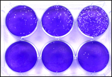
The plaque assay is the most direct way to count infectious virus: this is because, as a first and sensible approximation, each plaque is the product of one single infectious unit.
In a plaque assay, a series of virus dilutions is prepared, most typically 10-fold dilutions. These dilutions are then used to inoculate cell monolayers, which are then overlayed with a solid (e.g., agarose) or semisolid (e.g., carboxymethyl cellulose) overlay to prevent the cell-free spread of the newly released virus (limiting the infection to cell-to-cell spread). This is what gives shape to plaques (or foci, if the infection is visualised by immunostaining).
To determine the number of infectious units in the stock of interest, the number of plaques counted in one well is divided by the dilution factor of that well, and reported per millilitre by multiplying the obtained value by the fraction of millilitre that has been added to the well:
IU/ml = Number of plaques / dilution factor × (1 ml/inoculated volume)
So, for instance, if we count 32 plaques at the 10-3 dilution, and the cells were infected with 0.5 ml of that virus dilution, the number of infectious units/ml is calculated as:
32 plaques / 10-3 × 2 = 6.4 × 10⁵ infectious units (IU)/ml.
Cells can be counted in just one well, or at all dilutions where an accurate count is achievable (i.e., where there aren’t too many plaques touching each other, or too few plaques – below the limit of quantification), and these counts are averaged for higher accuracy.
Calculating the TCID50
Compared to the plaque assay, the TCID50 is a more indirect way to determine the number of infectious particles, as it includes a probabilistic assumption in the calculation: that at the dilution in which only 50% of the wells infected display CPE, only one virus particle is present. This is because, statistically, when only one virus particle is present, it can either infect or not infect; in other words, it has a 50% chance of infecting the cells.
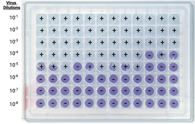
As in the plaque assay, a series of virus dilutions is prepared and used to inoculate cell monolayers in a 96-well plate format. The differences with the plaque assay are that multiple replicates are required for each dilution (generally 4 or more), and the virus is left free to spread through the media without constraints, as the ideal readout is complete CPE, rather than distinct plaques or foci.
Another difference is that calculations are less straightforward. Several calculation methods can be used to derive the virus concentration per milliliter starting from the limiting dilution. The most often used methods are the Reed-Muench method and the Spearmen-Karber method.
The Reed and Muench method
For a better understanding, let’s divide the process into six steps.
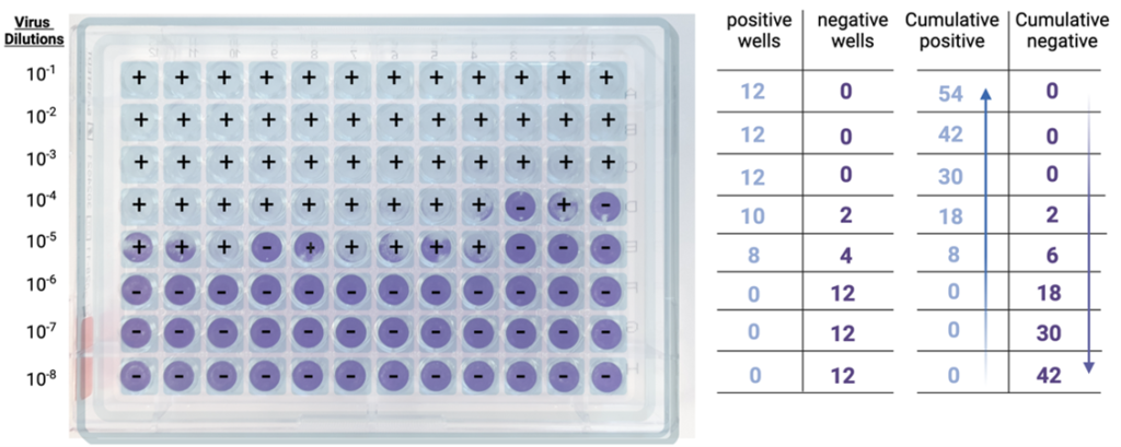
Step 1: Well scoring. For each dilution, positive wells (showing CPE) and negative wells (showing no CPE) are counted.
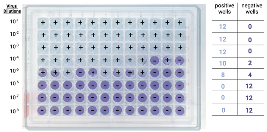
Step 2: Cumulative sums. Then, for each dilution, the cumulative sum of all positive wells is determined, by adding the number of positive wells at that dilution to the number of positive wells at all dilutions below (e.g., in the example below, at the 10-4 dilution, the cumulative sum is given by adding 10+8+0+0+0).
The cumulative sum of all negative wells is also determined, by adding the number of negative wells at that dilution to the number of negative wells at all dilutions above (e.g., in the example below, at the 10-4 dilution, the cumulative sum is given by adding 2+0+0+0).

Step 3: Infection rates. Cumulative positives and negatives are then used to calculate the infection rate for each dilution, which is obtained using the formula below:
Infection rate = Number of cumulative positive units / (number of cumulative positive units + number of cumulative negative units).
Back to our 10-4 dilution, the infection rate is 18/(18+2) = 0.9, or 90%.
At the 10-5 dilution, the infection rate is 8/(8+6) = 0.57, or 57%.
At the 10-6 dilution, the infection rate is 0/(0+18) = 0, or 0%.
Step 4: 50% Endpoint determination. Next, the dilutions that bracket the 50% infection rate are identified. In the example above, these two dilutions are 10-5, with an infection rate of 57% (the first value above 50%) and 10-6, with an infection rate of 0% (the first value below 50%).
Step 5. Proportionate Distance. The reason for calculating the proportionate distance (PD) is to pinpoint exactly where the 50% infection rate occurs between two dilutions.
Using the dilutions identified in Step 4 (57% and 0% in our example), we can calculate the proportionate distance using the following formula:
PD = (Infection rate above 50% – 50%) / (Infection rate above 50%) – (Infection rate below 50%).
In our example: (57% – 50%) / (57% – 0%) = 0.12
As an aside, if the exact 50% infection rate is obtained at a certain dilution, this simplifies the calculations and we won’t need to determine the PD, as this would be 0 [(50% – 50%) / (50% – X%) = 0].
Step 6. TCID50 determination. Finally, we are ready to calculate the TCID50 (hurray!), first as log (TCID50):
Log (TCID50) = log (dilution with infection rate above 50%) + (-PD) × log dilution factor.
In the example above: Log (TCID50) = -5 + (-0.12 × 1) = -5.12
From the log (TCID50) we can then compute the TCID50, which is ultimately expressed as the reciprocal of the dilution:
TCID50 = 105.12 = 1.3 × 10⁵
Finally (promised!), we just need to take into account the volume of inoculum used. If this was 0.1 ml, the TCID50 titer will be:
TCID50/ml = 1.3 × 105 × 10 = 1.3 × 10⁶/ml
The Spearman-Karber method
If the Reed-Muench method looks tricky, you’ll be pleased to know that the Spearman-Karber method is much simpler, as only a count of the total number of positive wells is required.
Experimentally, dilutions, infections, and counting of positive wells are performed in the same way as done for the Reed and Muench method.
Then, the log (TCID50) is calculated as:
Log (TCID50) = log (lowest dilution at which 100% CPE is observed) + I × [0.5 – (total number of wells displaying CPE/total number of replicate wells per dilution)].
“I” is the log of the dilution factor increments; in our case, we have a 10-fold increment, so that value will be 1.
Back to the example above:
Log (TCID50) = log (10-1) + 1 × [0.5 – (54/12)] = -1 + -4 = -5
TCID50 = 105 = 1.0 × 10⁵
TCID50/ml = 1.0 × 105 × 10 = 1.0 × 10⁶/ml.
Which method to use?
What are the advantages and disadvantages of these methods?
Clearly, the Spearman-Karber method, with much fewer calculation steps, is more straightforward and less prone to calculation errors. However, the Reed-Muench, by methodically calculating the infection rates at each dilution, provides a clearer visualisation of infection at each step, which can be beneficial for other analyses. On the contrary, the Spearman-Karber, by relying simply on the total number of infected wells, must assume that the distribution of infected wells follows a certain pattern, with infected wells progressively decreasing as the dilution series progresses. This is a fair assumption in a virus titration, but an assumption nonetheless.
While the titres generated by both methods in the example above are slightly different, they are sufficiently close to give us confidence that either can be used reliably, and the choice depends on personal preference or experimental requirements, including regulatory guidelines: while neither method is inherently superior to the other, some standard operating procedures (SOPs) or international standards may specify one method based on historical usage and validation data available.
Generally, for detailed analyses where it is important to understand infection dynamics across the dilution range, the Reed-Muench may be preferred; for simple routine titrations, an easier method like the Spearman-Karber may be chosen, as more immediate and less prone to mistakes.
Do titres obtained from a TCID50 assay and from a plaque assay match? Almost, but not completely, as they are conceptually and mathematically different. In our next blog, we explain how to move between the two and why.