Virologists spend an awful lot of time counting virus particles, in all sorts of ways, and for many sorts of reasons. But ‘not all that glitters is infectious’, when we’re counting virus particles.
In the previous article, we focused on quantifying active viruses – those capable of propagating infection. Today, we turn to a different kind of measurement: the total viral count, infectious and non-infectious alike.
Quantitative real-time polymerase chain reaction (qRT-PCR) is our precision tool for this task. qRT-PCR excels at measuring viral genomes with accuracy, but it doesn’t distinguish between particles that can cause infection and those that can’t; it’s like counting keys in a drawer, without knowing which still open locks.
But qRT-PCR’s total count proves valuable in many contexts. In diagnostics, the presence of viral genetic material alone tells us what we need – whether a patient carries the virus, infectious or not. Vaccine manufacturers track total particle counts to ensure their products contain sufficient immune-stimulating material. And in research, comparing total to infectious particles reveals viral strategies: like when dengue virus produces over a thousand non-infectious particles for each that’s infectious, it’s likely using these non-infectious decoys to distract the immune system.
Understanding the mathematics behind qRT-PCR helps us interpret these numbers with precision and context. Each calculation is a clue. In this post, we get into the math of qRT-PCR for virus quantification; what the technique measures, and why those numbers matter.
qRT-PCR for virus quantification: standard, test samples, and Ct values
In a typical qRT-PCR run, together with the samples of interest, we’ll include a serial dilution of a sample of a known number of viral genome copies, known as the “standard”. Both the standard and the test samples undergo several cycles of amplification, generally up to 40, and the outputs of the run are the so-called Ct (Cycle threshold) values.
At each cycle, assuming that the reaction is 100% efficient (more on this later), the amount of amplified DNA will double, as each piece of DNA in the reaction is duplicated. The Ct value is the cycle number at which the amplification products of a sample go above a certain detection threshold: the earlier this happens, the more abundant the sample was in the first place, and the lower the Ct will be. Therefore, the lower the Ct, the higher the starting amount in the sample.
Plotting the standard curve
Let’s now look at our standard. This is normally run over several dilutions (generally at least six 10-fold or 3-fold dilutions), and the Ct values relative to each point will increase as the samples become progressively less abundant.
It is common to plot the Ct values generated from each dilution of the standard on the y-axis of a graph, and the logarithm of the concentrations on the x-axis (Figure 1). The logarithmic scale is used because it helps distribute the data points evenly across the x-axis, as low concentrations would otherwise cluster together.
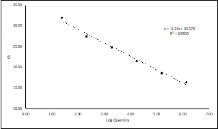
Figure 1: Example of a standard curve for virus quantification, with the log concentration on the x-axis and the Ct values on the y-axis. The curve has a negative slope, going from top left to bottom right, as there is an inverse correlation between target concentrations and Ct values.
Interpreting the Standard Curve
The curve generated in this graph is linear within a specific range of DNA concentrations: the linear part can be described as the interval between where the amount of DNA is too little or too great for the instrument to accurately quantify. When it’s linear, it’s ‘just right’.
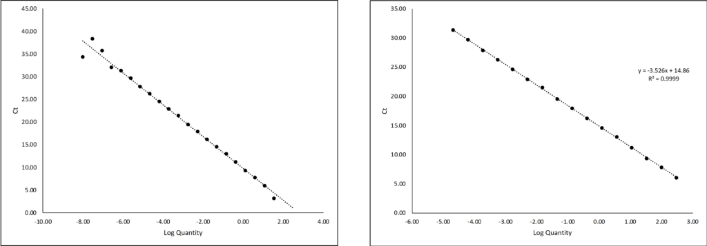
Figure 2: For the graph on the left, the five data points on the top left and the last point on the bottom right fall outside the linear range: here the samples are too dilute or too concentrated, respectively, to be accurately quantified. For the graph on the right, these values are removed and only the linear range is displayed.
During assay validation, the linear quantifiable range should be confirmed experimentally over several repeats. The lowest concentration that can be detected reproducibly over multiple runs is called the Limit of Detection (LoD), while the lowest concentration that can be quantified reliably over multiple runs is called the Limit of Quantification (LoQ).
Understanding the equation: slope and intercept
The equation of the curve generated from the standard in the linear range is expressed as:
y=mx+b
Rearranged, this curve allows us to determine the unknown amount of DNA in our test samples (x), from its determined Ct value (y):
x = (y-b)/m
In the equation, m represents the slope of the curve, and will be a negative value since there is an inverse relationship between Ct and concentration (the more abundant the target, the lower the Ct value).
The intercept, b, represents the Ct at which the curve touches the y-axis. When this happens, x=0, and because x=log10(concentration), for the definition of log10, we will have that 10x = (concentration) à 100 = 1. In other words, the intercept tells us the Ct corresponding to “1” of whichever unit we have in the x-axis.
Genome copies or mass
Therefore, if we were quantifying our genomes in mass, e.g., nanograms, the intercept would tell us the Ct value that corresponds to 1 nanogram. Then, the curve can continue beyond x=0, into the negative x values, since in a log scale these values simply correspond to fractions of a nanogram (e.g. 10-1 = 0.1 ng).
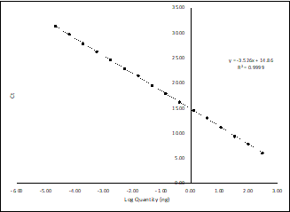
Figure 3: Standard curve extending beyond x=0, into fractions of nanograms.
However, if we are working in copy numbers (as in Figure 1), it’ll be different, as in this setting we can’t talk about a fraction of a genome copy: “1” is the minimal unit that we can quantify, and Ct values beyond that point are most likely artefacts.
In this context, let’s consider virus diagnostics. Imagine the highest concentration of our standard curve corresponds to 106 genome copies and has a Ct of 16. If the PCR reaction is 100% efficient, by halving the amount at each cycle, we would expect to reach 1 copy around cycle 35–36. So values obtained beyond this point would need to be considered noise.
This highlights the importance of the standard curve – not only does it allow us to quantify unknown samples, but it also informs us about the assay’s linear range, detection and quantification limits, and noise.
Linearity
The Ct values of the standard curve should appear equally spaced in the graph when plotted logarithmically, reflecting a linear relationship. For example, because the DNA in the reaction doubles at each cycle, each point of a 10-fold dilution series should be spaced about 3 cycles (3.3, to be precise) from the previous point.
We can also check how well our data is conforming to expectations by calculating the R2 value (coefficient of determination), which indicates how well the regression line fits the data. An R2 value above 0.99 is considered ideal, signifying strong linearity.
Efficiency
As mentioned earlier, 100% efficiency means that at each cycle, the amount of DNA doubles. Inefficiencies – due to reaction inhibitors, suboptimal primer design, or poor sample quality – are common in real-world assays. Efficiency (E) is calculated using the slope (m) value from the standard curve in the formula below:
E=[(10−1/m)−1]×100
For instance, if m=−3.57, then E=90.5%.
As a rule of thumb, efficiencies between 90% and 110% correspond to slopes between −3.3 and −3.6. Deviations beyond this range indicate problems that may need to be addressed before interpreting the results.
How can mathematics help us?
The numbers from qRT-PCR tell stories, if we can read them. Getting to know and understand Ct values, standard curves, efficiency, and linearity work helps ensure that the results generated (and conclusions drawn) are meaningful and reliable.
While qRT-PCR provides an invaluable means of quantifying viral genomes, it’s essential to recognise potential artefacts, particularly when it comes to copy numbers and noise.
Ultimately, familiarity with these concepts lets researchers and clinicians make informed decisions. And when we know how to optimise those parameters, we can make the assay more reliable and robust.

